Getting Started¶

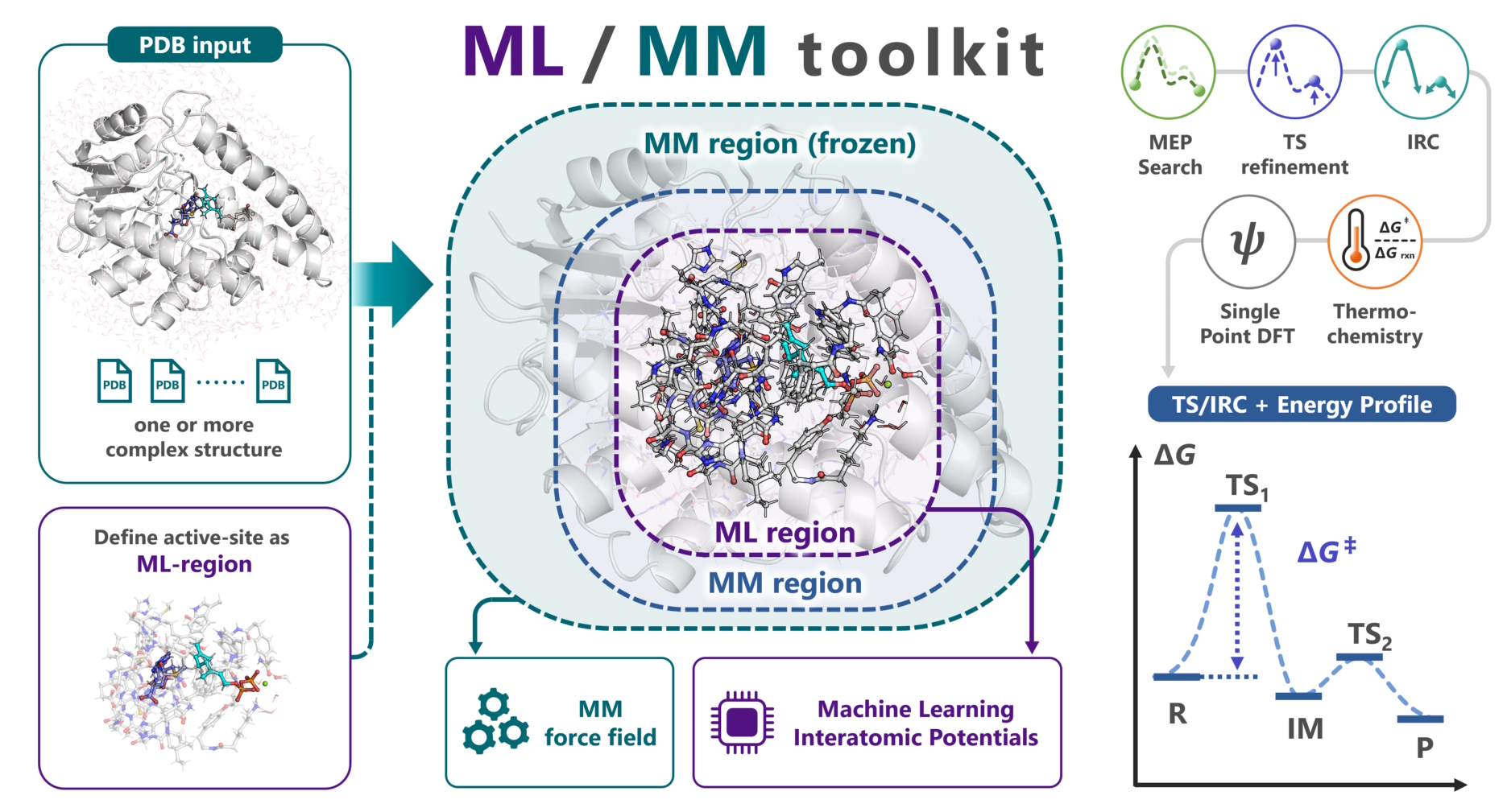
mlmm-toolkit is a Python command-line toolkit that uses ML/MM (machine learning / molecular mechanics) to search automatically for candidate enzyme reaction pathways, starting from PDB / mmCIF structures.

The reacting part of the enzyme (the ML region) is computed with a machine-learning interatomic potential (MLIP), and the protein around it with an Amber force field (MM). MLIPs are neural networks trained on DFT (density functional theory) data; they give energies and forces close to DFT accuracy at a much lower cost.

In many cases, a single command like this one gives a first draft of the reaction pathway:

mlmm -i 1.R.pdb 3.P.pdb -c 'SAM,GPP,MG' -l 'SAM:1,GPP:-3'

This page follows the steps of studying an enzyme reaction mechanism and explains the basics of computational chemistry and how to use mlmm-toolkit along the way.

Examples: the examples/beza/ directory holds the structures used above (1.R.pdb, 3.P.pdb) and a workflow script (MEP search and scan pipelines) built around the GPP C6-methyltransferase BezA (Tsutsumi et al., Angew. Chem. Int. Ed. 2022, 61, e202111217). After installation, get it with git clone https://github.com/t-0hmura/mlmm_toolkit && cd mlmm_toolkit/examples/beza and run the command above there.

Overall workflow¶

An enzyme reaction mechanism is studied in the seven steps below. mlmm-toolkit runs steps 2–6 in a row with one command.

Step	What you use	In `mlmm-toolkit`
1. Prepare the complex structure	Structure prediction or docking → MD	Outside `mlmm-toolkit`
2. Build the ML region and layers	`extract`, `mm-parm`, `define-layer`	`extract` and `define-layer` with `-c`; `mm-parm` without `--parm7`
3. Find the reaction pathway	`scan`, `path-opt`, `path-search`	`scan` with `-s`; the path search in every mode except TS-only mode
4. Optimize the TS and check the imaginary mode	`tsopt`	With `--tsopt`
5. Check that the TS connects R and P	`irc`	With `--tsopt`
6. Compare the energies	`freq`, `dft`	With `--tsopt` plus `--thermo` / `--dft`
7. Make an overall judgment	Fraction of reactive arrangements (NAC), minimum and median barriers	Over several snapshots

This command runs all of steps 2–6:

mlmm -i 1.R.pdb 3.P.pdb -c 'SAM,GPP,MG' -l 'SAM:1,GPP:-3' --tsopt --thermo --dft

Each step also runs on its own as a subcommand (extract, mm-parm, define-layer, tsopt, irc, and so on; see the subcommand list).

1. Prepare the complex structure¶

Build a structure of the enzyme–substrate complex with structure prediction such as AlphaFold 3, Boltz-2, or OpenFold3, or with a docking tool. Run molecular dynamics (MD) on it and take snapshots of various conformations. The Amber topology used in the MD can be reused with --parm7. Rather than drawing a conclusion from one structure, compute several snapshots.

For the structures you give mlmm-toolkit, watch these three points.

Add hydrogens (required)¶

Input structures must contain every hydrogen atom; all does not add them. When a structure lacks hydrogens (a crystal structure, for example), add them beforehand with a tool such as these:

Recommended tool	Example command	Notes
reduce (Richardson Lab)	`reduce input.pdb > output.pdb`	Fast; widely used to add hydrogens to crystal structures
pdb2pqr	`pdb2pqr --ff=AMBER --pdb-output=output.pdb input.pdb output.pqr`	Adds hydrogens (use `output.pdb`)
Open Babel	`obabel input.pdb -O output.pdb -h`	General-purpose cheminformatics toolkit
mm-parm --add-h	`mlmm mm-parm -i input.pdb --add-h`	Adds hydrogens with PDBFixer at `--ph` (default 7.0)

all fills blank element columns (77–78) by itself; before a standalone command such as extract, fill them with add-elem-info. If the PDB has alternate locations (altLoc), keep one per residue with fix-altloc.

Keep the same atom order (multiple structures)¶

When the input has several structures, such as a reactant (R) and a product (P), every structure must list the same atoms in the same order (only the coordinates differ). Run the hydrogen tool on every structure with the same settings, and in PyMOL tick Original atom order when saving. An atom that moves to another residue keeps its residue and atom name from R: in the bundled example, the hydrogen that GPP passes to Glu186 is still H11 of GPP 321 in 3.P.pdb.

Match `-l` to the hydrogens¶

Give each ligand the charge that matches the hydrogens in the file. In the bundled example, SAM has 23 hydrogens, so it is SAM:1; with 22 hydrogens it would be SAM:0. When the charge and the hydrogens do not match, mm-parm stops with an electron-count error before it runs antechamber.

mmCIF (.cif, .mmcif) and PDB files beyond the fixed-column limits of the PDB format work with all and the calculation commands; the standalone mm-parm reads PDB only. See mmCIF input for details.

2. Build the ML region and layers¶

An enzyme has thousands to tens of thousands of atoms, too many to compute entirely with DFT. Instead, only the reacting part is computed with an accurate method, and the protein around it with a light molecular mechanics (MM) force field. Computing the reacting part with quantum chemistry (QM) is the QM/MM method; replacing that QM with an MLIP gives ML/MM. mlmm-toolkit combines the two calculations by the ONIOM subtraction:

E_total = E_REAL_low + E_MODEL_high - E_MODEL_low

REAL is the full system and MODEL the ML region; high is the MLIP, and low is the MM backend. The full system is computed with MM, the ML region with both the MLIP and MM, and the MM energy of the ML region is subtracted so that it is not counted twice.

ML region: all takes as the ML region the residues with an atom within -r (default 2.6 Å) of the substrates given with -c.
Link atoms: where the boundary between the ML region and MM cuts a covalent bond, the ML-region calculation caps the ML side of the cut bond with a hydrogen (a link hydrogen). The link hydrogen sits along the cut bond, and the force on it is passed back to the atoms on both sides. mlmm-toolkit places the link hydrogens automatically (ML/MM Calculator).
MM layers: mm-parm builds the Amber topology of the full system, and define-layer splits the atoms outside the ML region into Movable-MM, which moves during optimizations, and Frozen-MM farther out, which stays fixed. The layers are stored in the B-factor column of the PDB.

See Building the ML region and layers for details.

Compared with a cluster model: a cluster model cuts out only the part involved in the reaction, so to keep the shape and environment of the protein it needs a large model that also holds residues not directly involved in the reaction. ML/MM keeps the surrounding protein as MM, so the ML region is easier to shrink to just the reacting part, and the calculation can be lighter than with a cluster model. In the bundled example, the default ML region has 632 atoms; moving the main-chain atoms to MM gives 397 atoms, and picking the residues yourself gives 129 atoms (Shrink the ML region).

Size of the ML region: in a study of COMT (catechol O-methyltransferase) that varied the size of the QM region in QM/MM, adding residues in order of distance from the substrate made the activation energy nearly constant at about 500–600 atoms (Kulik et al., J. Phys. Chem. B 2016, 120, 11381). When you pin down barrier values, check that enlarging the ML region does not change the result. When a residue involved in the reaction is missing, raise -r or add the residue to -c or --selected-resn (Make the model larger).

3. Find the reaction pathway¶

Optimize the reactant (R) and product (P) structures, and search for the minimum energy path (MEP) that connects R and P. The highest-energy point on the path is the candidate for the transition state (TS). This step is the same as in a reaction-mechanism study of small molecules.

There are three ways to give the input:

Mode	Input	What happens
Endpoint mode	Two or more PDBs (`-i R.pdb P.pdb`)	Builds the ML region and layers from the structures and searches the MEP
Scan-list mode	One PDB + `--scan-lists` (`-s`)	Drives the chosen distances, angles, or dihedrals step by step to build the pathway
TS-only mode	One PDB + `--tsopt`	Skips the MEP search and goes straight to optimizing the TS candidate and running IRC

Note: a single-structure input needs either --scan-lists/-s or --tsopt.

4. Optimize the TS and check the imaginary mode¶

A TS is a point where the energy is a maximum along the direction in which the reaction proceeds and a minimum along every other direction (a first-order saddle point). A frequency calculation at this point gives an imaginary frequency (an imaginary mode) for the reaction direction only. If n_imag (the number of imaginary modes) is 0, the point is a minimum; if it is 2 or more, the point is not a TS.

A successful TS optimization gives one imaginary mode along the reaction coordinate. Also check that this mode moves the intended bonds that form and break.

Frozen atoms and PHVA: when atoms are frozen, as in Frozen-MM, the energy is neither a minimum nor a saddle point along the directions that move the frozen atoms. A frequency calculation over all atoms can therefore show imaginary modes that come only from the freezing. Instead, the frequencies are taken from the Hessian (the second derivative of the energy) of the movable atoms only. This is called partial Hessian vibrational analysis (PHVA), and freq in mlmm-toolkit runs it over the ML region and the Movable-MM atoms.

5. Check that the TS connects R and P¶

One imaginary mode does not guarantee that the TS lies between the intended R and P. The IRC (intrinsic reaction coordinate) goes downhill from the TS to both sides; check that it ends at the intended R and P. mlmm-toolkit also optimizes both IRC endpoints, so even if the IRC stops partway, the result is usable when the endpoint optimizations reach the intended R and P.

6. Compare the energies¶

--thermo adds the thermochemical correction (Gibbs free energy) from vibrational analysis, and --dft adds DFT single points; with them you get the activation energy (R → TS) and the reaction energy (R → P).

When the run finishes, the output directory (-o, default ./result_all/) contains the following files. Output Directory Layout lists the main files, and JSON Output Reference every key of summary.json.

File / folder	Contents
`summary.log`	Text summary (directory layout and progress of each stage)
`summary.json`	Machine-readable results (barriers, energies of each state, bond changes)
`energy_diagram_*.png`	Energy profile plots (electronic energy / Gibbs-corrected)
`mep_trj.pdb` / `mep_trj.cif`	Animated trajectory of the minimum energy path (MEP)
`ml_region.pdb`, `mm_parm/`, `layered/`	The ML region, the full-system Amber topology, and the layered full-system PDBs; reuse them with `--model-pdb` and `--parm7`
`segments/seg_NN/`	Detailed results for each reaction segment (optimized R/TS/P structures, IRC trajectories, and more; with `--tsopt`)

At the end of the terminal output, the Scientific status: line under ====== Pipeline summary ====== (scientific_status in summary.json) is success when every requested stage converged, otherwise partial or failed with the reasons in scientific_status_reasons. Whether the TS has n_imag = 1 and the endpoints are the intended R and P is for you to check; each quickstart lists the files to open.

7. Make an overall judgment¶

One pathway is not enough for a conclusion. Judge whether the mechanism is plausible by looking together at how often reactive arrangements appear in the MD (near-attack conformations, NACs: the reacting atoms are close and oriented to react) and at the minimum and median barriers over several snapshots.

The results depend strongly on the starting structure and on how the model is built, so trial and error, recomputing with other structures and models, cannot be avoided. mlmm-toolkit automates steps 2–6 and computes them fast with MLIPs, so it suits this trial and error.

Going further¶

mlmm-toolkit is especially useful for high-throughput calculations over many substrates or mutants, for supporting experimental results, and for trial and error.

MD of the whole system with an MLIP, or ML/MM MD, also shows the dynamics of the whole enzyme. These MD runs cost more than cluster-model or ML/MM calculations on the potential energy surface, so a good approach is to run them after mlmm-toolkit has confirmed the mechanism.

MLIPs are a fairly new technology, so for a purely computational paper, DFT calculations will probably still be expected for a while. mlmm-toolkit also has a DFT backend, so everything up to QM/MM (DFT/MM) calculations, with the ML region computed by DFT, stays within one tool (Refine an MLIP TS with DFT). Give it a try.

Where to start¶

For environment setup, see the Installation guide.

Try it in a web browser: the Colab GUI notebook (pick the ML region in 3D)
Start from several PDB structures: Quickstart: mlmm all
Explore from one PDB structure with a scan: Quickstart: mlmm all --scan-lists
Optimize and check a TS candidate: Quickstart: TS-only mode

How the command works¶

Installation provides the mlmm command. Without a subcommand, all runs.

# These two do the same thing
mlmm [OPTIONS]...
mlmm all [OPTIONS]...

Choosing between all and individual commands¶

Use all to run model setup → MEP search → TS optimization and IRC → frequencies and DFT in one command, or while you are still exploring and want one command to manage the outputs.
Use the individual commands to run each stage in turn and check its result before the next; for a complex reaction, this often works better than one all run. They also fit a custom sequence and a run that reuses the parm7 and layered PDB of an earlier run.

The individual ML/MM commands need the full-system topology (--parm7) and the ML region (--model-pdb, --model-indices, or the B-factor layers of the input); all builds both. -q is the charge of the ML region, not of the whole system. See ML/MM options.

Main CLI options¶

Option	Example	Description
`-i, --input`	`1.R.pdb 3.P.pdb`	Input structure files (PDB / mmCIF); accepts several
`-c, --center`	`'SAM,GPP'` / `'A:SAM:123'`	Extraction center (substrate residue names, residue IDs, or a PDB file); the ML region is cut out around it. Without it, no extraction runs, the whole structure is used, and the ML region comes from the B-factor layers or `--model-pdb` (with neither, the run stops with an error)
`-l, --ligand-charge`	`'SAM:1,GPP:-3'`	Formal charge of each ligand, as a mapping (standard residues and ions are counted automatically)
`-q, --charge`	`-2`	Total charge of the ML region, not of the whole system (set it to override the automatic value)
`-m, --multiplicity`	`1`	Spin multiplicity (default `1`, a singlet)
`--parm7`	`real.parm7`	Full-system Amber topology to reuse, such as one from an earlier run or from the MD that produced the input snapshot; skips `mm-parm`
`--model-pdb`	`ml_region.pdb`	ML region as a PDB; takes precedence over `-c` and the B-factor layers
`--tsopt/--no-tsopt`	(flag)	Turns on TS optimization and IRC
`--thermo/--no-thermo`	(flag)	Runs vibrational analysis and thermochemical correction with the QRRHO (quasi-rigid-rotor harmonic oscillator) model (with `--tsopt`)
`--dft/--no-dft`	(flag)	Runs DFT single points on the resulting structures (with `--tsopt`)
`-b, --backend`	`uma` / `orb` / `mace`	Backend for the ML region (default `uma`; `dft` is also available)

For the syntax rules, see Common options and selectors; for every option, see the all CLI reference.

AI agent skills¶

mlmm-toolkit ships instructions for AI agents (Claude Code, Codex, Cursor, and others) in the skills/ directory. To install them, tell your AI agent:

Import https://github.com/t-0hmura/mlmm_toolkit/tree/main/skills as skills, and install mlmm-toolkit by following mlmm-install.

If you cloned the GitHub repository, you can give the local skills/ path instead. Then you can ask, for example:

Read the paper, build a model from the PDB structure PDB ID, and study the mechanism of the reaction step with the mlmm-toolkit skills.

The skills cover the CLI subcommands, structure input and output, backend installation, TS search strategy, and HPC runs. Load skills/ into an agent, and it can run and analyze calculations from plain-language instructions. For where to place the files and the full list of skills, see Skills for AI Agents.

Troubleshooting and support¶

If an error occurs during a run, see these pages:

Troubleshooting: fixes by error symptom, and solutions for installation and environment problems
MLIP Backends: choosing a backend and running parallel workers; Device Configuration & HPC Setup for GPU memory, device settings, and job scripts on clusters

To see every option of a command, use the help options:

mlmm <subcommand> --help
mlmm all --help-advanced

Report unresolved problems and bugs on GitHub Issues.